Common Root Cells
Multi-branch dataset with common root cells
Priyansh Srivastava
Source:vignettes/Common-Root-Cells.Rmd
Common-Root-Cells.RmdIntroduction
scMaSigPro is designed to handle datasets with at least
two branches and requires that cells be assigned exclusively to these
branches. This vignette demonstrates how to evaluate datasets with
common root cells using the scMaSigPro approach. We will
utilize an object from Monocle3’s newCellDataSet
class in this analysis.
Installation
Currently, scMaSigPro is available on GitHub and can be
installed as follows:
Bioconductor and Dependencies
# Install Dependencies
if (!requireNamespace("BiocManager", quietly = TRUE))
install.packages("BiocManager")
BiocManager::install(version = "3.14")

BiocManager::install(c('SingleCellExperiment', 'maSigPro', 'MatrixGenerics', 'S4Vectors'))
scMaSigPro latest version
To install scMaSigPro from GitHub, use the following R
code:
# Install devtools if not already installed
if (!requireNamespace("devtools", quietly = TRUE)) {
    install.packages("devtools")
}

# Install scMaSigPro
devtools::install_github("BioBam/scMaSigPro",
                         ref = "main",
                         build_vignettes = FALSE,
                         build_manual = TRUE,
                         upgrade = "never",
                         force = TRUE,
                         quiet = TRUE)
Setup
We will start by loading the necessary libraries.
## For plotting
library(scMaSigPro)
library(ggplot2)
## Install and load 'monocle3-1.3.4'
library(monocle3)
Simulated Data
For this vignette, we will use a simulated dataset containing 1,977
cells and 501 genes. The dataset was generated using the Dyntoy package
and is sourced from the tradeSeq
repository. This dataset has been simulated to have three branches
and is analyzed with Monocle3 (version 1.3.4).

In the figure-A, we can see that the cells share a common root and
then diverge into multiple branches. The cells first diverge into two
branches and then into three branches. Figure B illustrates the elements
of the trajectory used as input in scMaSigPro for the
common root cells setup.
Hard Assignment of Cells
An important prerequisite for using scMaSigPro is the
hard assignment of cells to branches. This means that each cell must be
exclusively assigned to one branch. There are broadly two ways to assign
cells:
- Hard assignment (0 and 1), where each cell belongs to only one branch.
- Soft assignment (0 to 1), where a cell can belong to multiple branches simultaneously.
In Monocle3, each cell is associated with only one branch, implying a
hard assignment, which is suitable for scMaSigPro current
version. On the other hand, tradeSeq can handle both hard
and soft assignments. In Slingshot, for instance, cells can be part of
multiple branches, which is a form of soft assignment. One key
difference is that Slingshot assigns different pseudotimes to each
branch, whereas Monocle3 uses a universal pseudotime for all
branches.
Extracting Assignmnet
Extracting Branch Assignments
We will follow the steps from the tradeSeq
Vignette to extract the assignment of cells to branches. However,
for the sake of simplicity, we will tweak these steps to avoid using the
magrittr and monocle3 packages. Instead, we will use base R functions
and directly access the S4 slots. 1
# Get the closest vertices for every cell
y_to_cells <- as.data.frame(cds@principal_graph_aux$UMAP$pr_graph_cell_proj_closest_vertex)
y_to_cells$cells <- rownames(y_to_cells)
y_to_cells$Y <- y_to_cells$V1

## Root Nodes
root <- cds@principal_graph_aux$UMAP$root_pr_nodes

## Extract MST (PQ Graph)
mst <- cds@principal_graph$UMAP

## All end-points
endpoints <- names(which(igraph::degree(mst) == 1))

## Root is also an endpoint so we remove it
endpoints <- endpoints[!endpoints %in% root]

## Extract
cellAssignments_list <- lapply(endpoints, function(endpoint) {
  # We find the path between the endpoint and the root
  path <- igraph::shortest_paths(mst, root, endpoint)$vpath[[1]]
  path <- as.character(path)
  # We find the cells that map along that path
  df <- y_to_cells[y_to_cells$Y %in% path, ]
  df <- data.frame(weights = as.numeric(colnames(cds@assays@data@listData$counts) %in% df$cells))
  colnames(df) <- endpoint
  return(df)
})

## Format
cellAssignments <- do.call(what = "cbind", cellAssignments_list)
cellAssignments <- as.matrix(cellAssignments)

# Update columns
rownames(cellAssignments) <- colnames(cds@assays@data@listData$counts)
head(cellAssignments[c(20:30), ])
## Y_1 Y_15 Y_18 Y_52 Y_65
## C20 0 0 0 1 0
## C21 1 1 1 1 1
## C22 0 0 0 1 0
## C23 0 0 0 1 0
## C24 0 0 0 1 1
## C25 1 0 1 0 0
scMaSigPro object
For this vignette, we will only consider three paths: the root, Y_18, and Y_15 (Refer Figure-A). We will remove the other paths and any cells that are part of those paths.
# Subset for 3 paths
cellAssignments <- cellAssignments[, c("Y_18", "Y_52", "Y_15"), drop = FALSE]

# Remove any of the cells which is not assigned to any path
cellAssignments <- cellAssignments[rowSums(cellAssignments) != 0, ]

# Create Cell Data
cellData <- data.frame(
  cell_id = rownames(cellAssignments),
  row.names = rownames(cellAssignments)
)

# Extract counts
counts <- cds@assays@data@listData$counts

# Subset counts
counts <- counts[, rownames(cellAssignments), drop = FALSE]
Creating Cell Metadata
Another important step is to label the elements (Refer to Figure-B). If a cell belongs to the root, then it is part of all the paths. If a cell is part of a link branch, then it is part of both the “Y_15 and Y_18” branches.
# Create Cell Metadata
cellData[["group"]] <- apply(cellAssignments, 1, FUN = function(x) {
  npath <- length(names(x[x == 1]))
  if (npath == 3) {
    return("root")
  } else if (npath == 2) {
    return(paste(names(x[x == 1]), collapse = "_links_"))
  } else {
    return(names(x[x == 1]))
  }
})
table(cellData[["group"]])
##
## root Y_15 Y_18 Y_18_links_Y_15 Y_52
## 453 307 676 43 498
# Extract from CDS
ptimes <- cds@principal_graph_aux$UMAP$pseudotime

# Remove cells which are not assigned to any path
ptimes <- ptimes[rownames(cellAssignments)]

# Assign to cellData
cellData[["m3_pseudotime"]] <- ptimes
Creating Object
# Create Object
multi_scmp_ob <- create_scmp(
  counts = counts,
  cell_data = cellData,
  ptime_col = "m3_pseudotime",
  path_col = "group",
  use_as_bin = FALSE
)
multi_scmp_ob
## Class: ScMaSigProClass
## nCells: 1977
## nFeatures: 501
## Pseudotime Range: 0 62.806
## Branching Paths: root, Y_15, Y_52, Y_18, Y_18_links_Y_15Each Branch as a Group (Approach-1)
The first approach to using scMaSigPro to analyze
branches with common cells is to consider the common cells as a separate
group. For the interpretation we will evaluate whether a particular
gene’s expression in the common root cells and it’s downstream branch is
similar.
Perform Binning
## Pseudotime based binning
multi_scmp_ob_A <- sc.squeeze(multi_scmp_ob)

## Plot bin information
plotBinTile(multi_scmp_ob_A)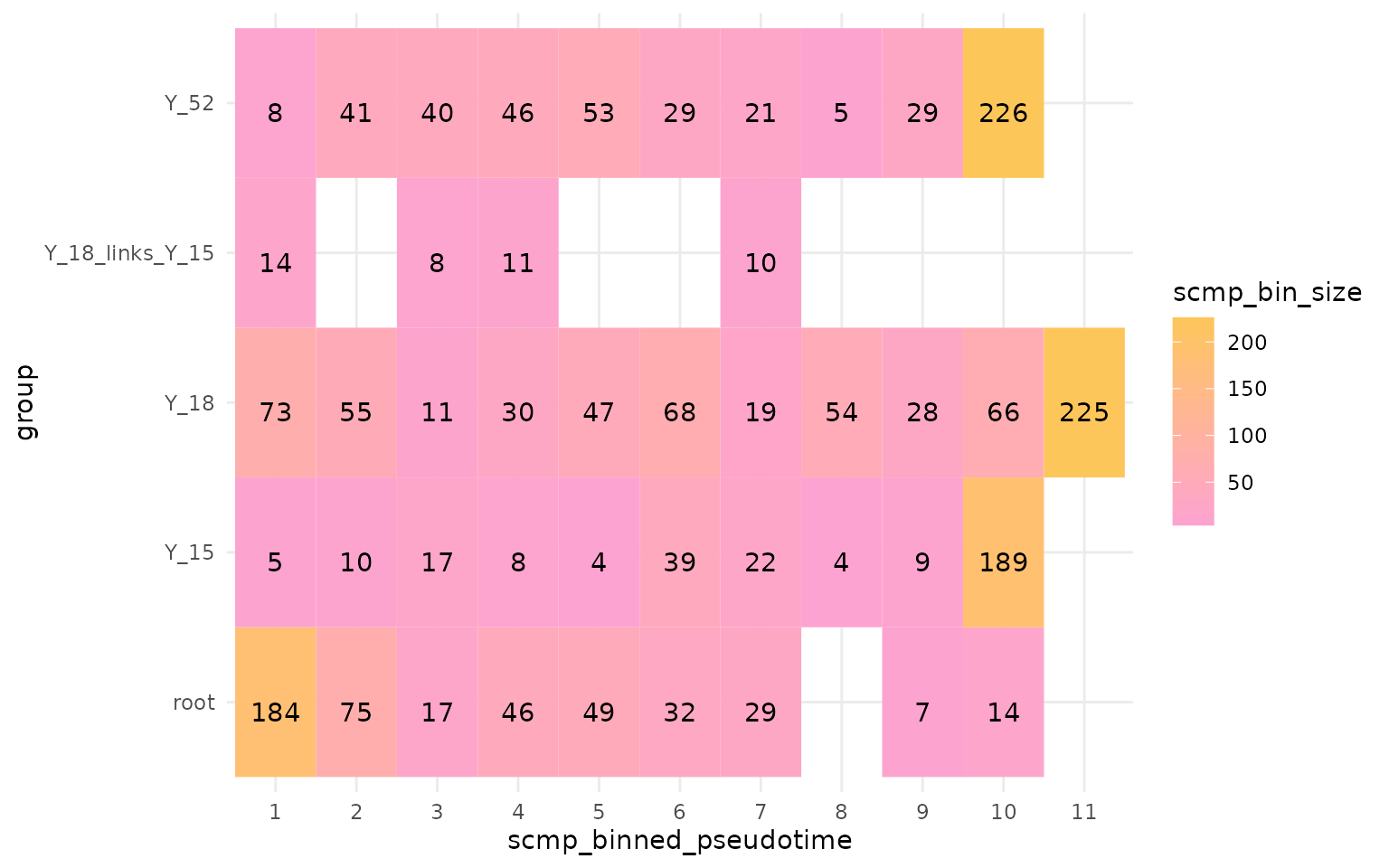
In the above figure, we can see that scMaSigPro
considers each group as a separate branch. Running
scMaSigPro with this configuration will lead to a different
interpretation of the data. This will help us evalute whether the
expression changes across branches compared to root. If you want to
consider the common root cells and branches together, you can follow the
next section.
Additionally, we can see that the common root cells and the resulting branches have the same values of binned pseudotime values. This is because the binning is performed independently over each branch.
Running Workflow
# Polynomial Degree 2
multi_scmp_ob_A <- sc.set.poly(multi_scmp_ob_A, poly_degree = 3)

# Detect non-flat profiles
multi_scmp_ob_A <- sc.p.vector(
  multi_scmp_ob_A,
  verbose = FALSE
)

# Model refinement
multi_scmp_ob_A <- sc.t.fit(
  multi_scmp_ob_A,
  verbose = FALSE
)

# Apply filter
multi_scmp_ob_A <- sc.filter(
  scmpObj = multi_scmp_ob_A,
  rsq = 0.55,
  vars = "groups",
  intercept = "dummy",
  includeInflu = TRUE
)

# Plot upset
plotIntersect(multi_scmp_ob_A)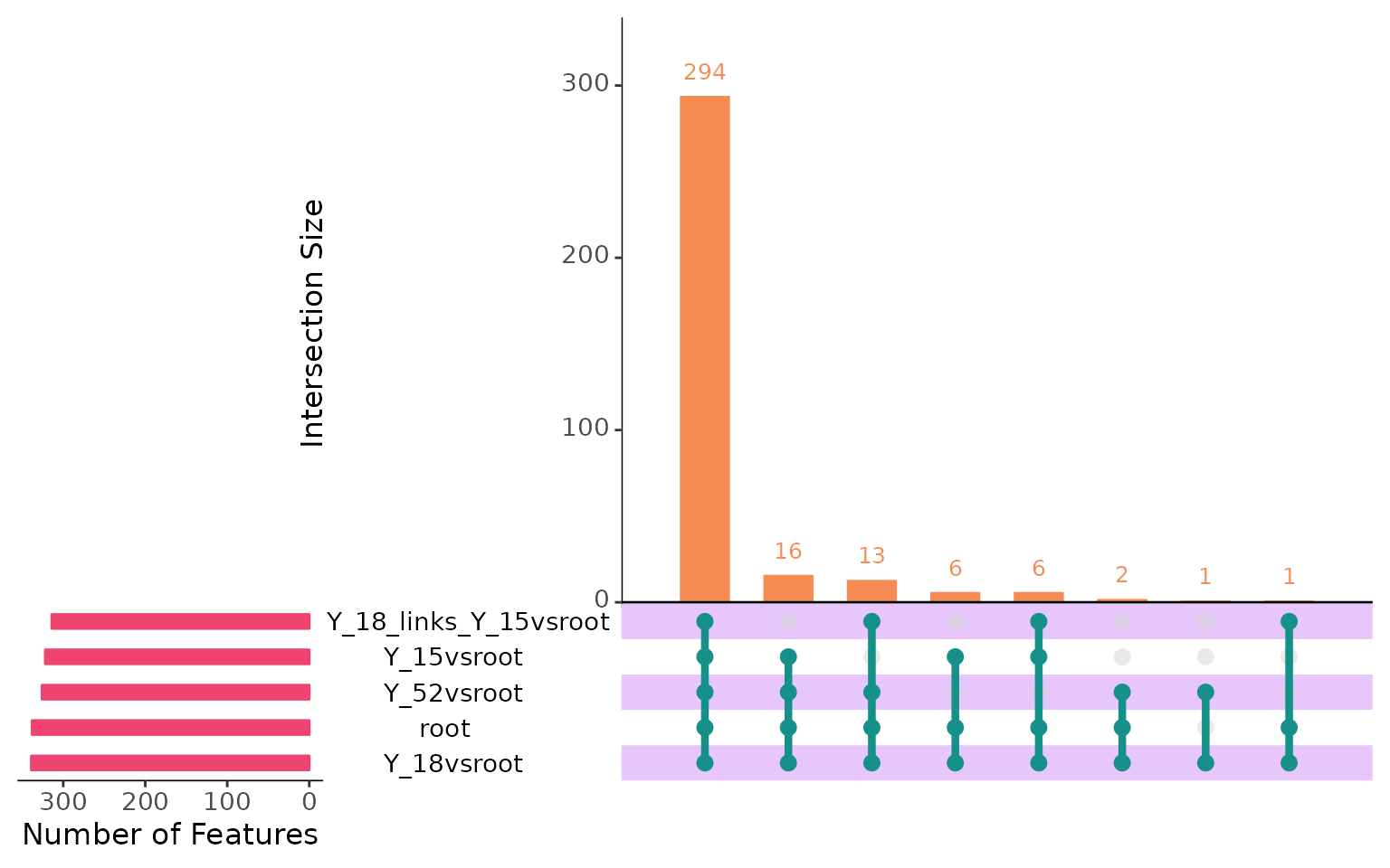
In the upset plot above, we can see that there are 294 genes which change among branches and also change with pseudotime. We will explore them later. First, let’s look at the genes that have similar expression in the “root”, “Y_18_links_Y_15vsroot” (link) and “Y_18” (branch).
scMaSigPro treated the “root” as the reference for all
branches. Let’s extract the intersection information from the
scMaSigPro object. Starting from scMaSigPro
version 0.0.4, the
plotIntersect(return = TRUE) function can be used to
extract the intersection information from the object as a dataframe.
Significant Genes
shared_genes <- plotIntersect(multi_scmp_ob_A, return = TRUE)
head(shared_genes)
## Y_15vsroot Y_18vsroot Y_18_links_Y_15vsroot Y_52vsroot root
## G3 1 1 1 1 1
## G7 1 1 1 1 1
## G9 1 1 1 1 1
## G10 1 1 1 1 1
## G11 1 1 1 1 1
## G12 1 1 1 1 1
## Similar expression in root, "Y_18_links_Y_15vsroot" and "Y_15"
gene_br_Y_15 <- rownames(shared_genes[shared_genes$Y_52vsroot == 1 &
  shared_genes$Y_18vsroot == 1 &
  shared_genes$Y_15vsroot == 0 &
  shared_genes$root == 1 &
  shared_genes$Y_18_links_Y_15vsroot == 0, ])
plotTrend(multi_scmp_ob_A, feature_id = "G42", points = F, lines = T)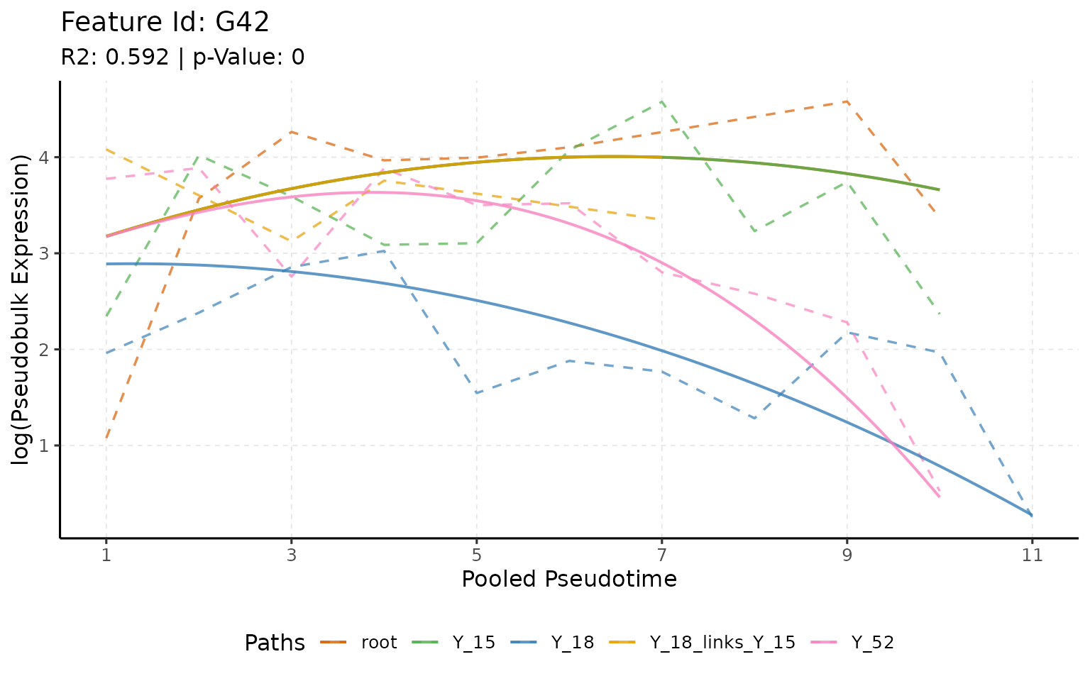
In the above plot, we can see that the gene G42 has a similar
expression in the “root”, “Y_18_links_Y_15vsroot,” and “Y_15.”. This is
a good example of how scMaSigPro can be used to identify
genes that are showing similar patterns in the common root cells and how
different is it in other branches. The main idea is to set the root as a
reference and then compare the branches to the root.
Next we can explore the 294 genes that we have in the intersection. As it is hard to see them all at once, we will first perform clustering and then look at them in groups.
## Perform Clustering
multi_scmp_ob_A <- scMaSigPro::sc.cluster.trend(multi_scmp_ob_A)

# Plot Clusters
plotTrendCluster(multi_scmp_ob_A, verbose = FALSE, loess_span = 0.8)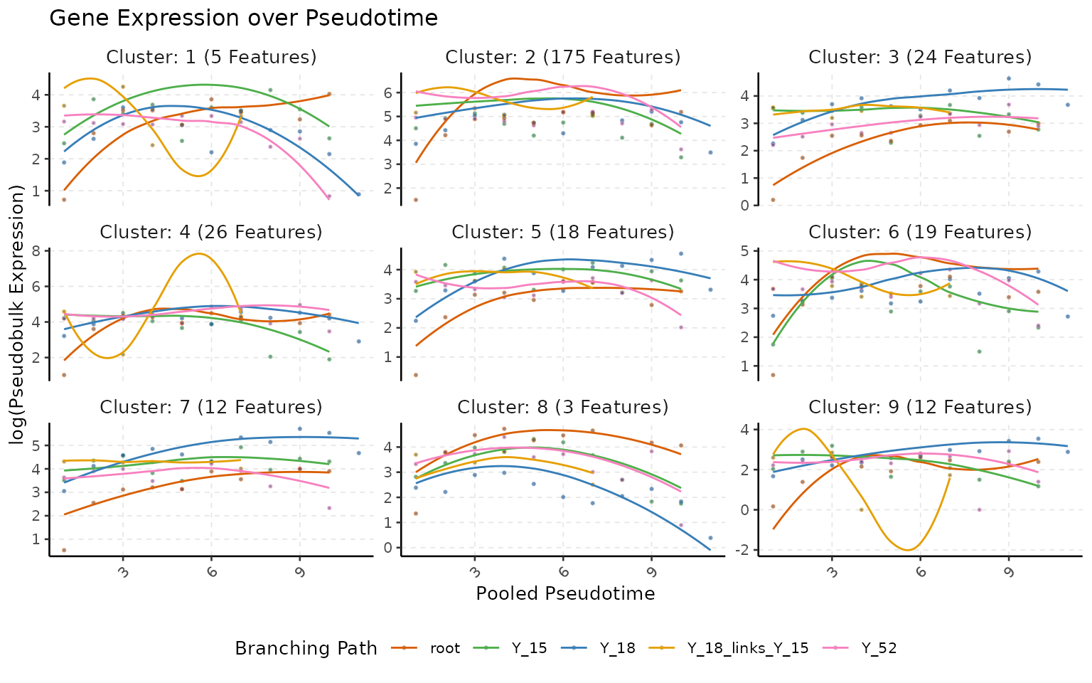
Ordering Common Cells (Approach-2)
Another approach is to reorder the pseudotime bins, meaning the bins representing the common root cells are ordered first, followed by the bins of the branches. This helps compare the gene expression of the common root cells togther with the downstream branches.
Reorder Bins Manually
Extract Binned Data
##            scmp_binned_pseudotime   scmp_bin group scmp_bin_size scmp_l_bound
## root_bin_1                      1 root_bin_1  root           184         0.00
## root_bin_2                      2 root_bin_2  root            75         2.22
## root_bin_3                      3 root_bin_3  root            17         4.45
## root_bin_4                      4 root_bin_4  root            46         6.67
## root_bin_5                      5 root_bin_5  root            49         8.90
## root_bin_6                      6 root_bin_6  root            32        11.10
##            scmp_u_bound
## root_bin_1         2.22
## root_bin_2         4.45
## root_bin_3         6.67
## root_bin_4         8.90
## root_bin_5        11.10
## root_bin_6        13.30
Create Bin Data for Root + Y_52
The main idea is to update the values in the binned pseudotime column using an offset. Based on our dataset, we observe that Y_52 is a branch that directly originated from the Root. Therefore, the bins of the Y_52 branch should be aligned right after it. This means that the offset for the Y_52 branch will be the maximum value of the binned pseudotime of the root branch.
## Create a new df
Y_52_binned_data <- binned_data[binned_data$group %in% c("root", "Y_52"), , drop = FALSE]

## Calculate Offset (Max Value of the root)
Y_52_offset <- max(Y_52_binned_data[Y_52_binned_data$group == "root", "scmp_binned_pseudotime"])

## Add offset
Y_52_binned_data[Y_52_binned_data$group == "Y_52", "scmp_binned_pseudotime"] <- Y_52_binned_data[Y_52_binned_data$group == "Y_52", "scmp_binned_pseudotime"] + Y_52_offset

## Update bins and rownames
Y_52_binned_data$group2 <- "Y_52"
rownames(Y_52_binned_data) <- paste(Y_52_binned_data$group2, Y_52_binned_data$scmp_binned_pseudotime, sep = "_bin_")

head(Y_52_binned_data[, -2])
## scmp_binned_pseudotime scmp_bin group scmp_bin_size scmp_l_bound
## Y_52_bin_1 1 root_bin_1 root 184 0.00
## Y_52_bin_2 2 root_bin_2 root 75 2.22
## Y_52_bin_3 3 root_bin_3 root 17 4.45
## Y_52_bin_4 4 root_bin_4 root 46 6.67
## Y_52_bin_5 5 root_bin_5 root 49 8.90
## Y_52_bin_6 6 root_bin_6 root 32 11.10
## scmp_u_bound group2
## Y_52_bin_1 2.22 Y_52
## Y_52_bin_2 4.45 Y_52
## Y_52_bin_3 6.67 Y_52
## Y_52_bin_4 8.90 Y_52
## Y_52_bin_5 11.10 Y_52
## Y_52_bin_6 13.30 Y_52Create Bin Data for Root + Link + Y_15|Y_18
For the other branches we will add an offset of both “link” and “Y_15|Y_18”.
## Create a new df
Y_18_binned_data <- binned_data[binned_data$group %in% c("root", "Y_18_links_Y_15", "Y_18"), , drop = FALSE]
Y_15_binned_data <- binned_data[binned_data$group %in% c("root", "Y_18_links_Y_15", "Y_15"), , drop = FALSE]

## Calculate Offset (Max Value of the root and Link)
Y_18_root_offset <- max(Y_18_binned_data[Y_18_binned_data$group == "root", "scmp_binned_pseudotime"])
Y_18_link_offset <- max(Y_18_binned_data[Y_18_binned_data$group == "Y_18_links_Y_15", "scmp_binned_pseudotime"])

## Add link offset to branch Y_18
Y_18_binned_data[Y_18_binned_data$group == "Y_18", "scmp_binned_pseudotime"] <- Y_18_binned_data[Y_18_binned_data$group == "Y_18", "scmp_binned_pseudotime"] + Y_18_link_offset
Y_15_binned_data[Y_15_binned_data$group == "Y_15", "scmp_binned_pseudotime"] <- Y_15_binned_data[Y_15_binned_data$group == "Y_15", "scmp_binned_pseudotime"] + Y_18_link_offset

## Add root offset to (link+ branch)
Y_18_binned_data[Y_18_binned_data$group != "root", "scmp_binned_pseudotime"] <- Y_18_binned_data[Y_18_binned_data$group != "root", "scmp_binned_pseudotime"] + Y_18_root_offset
Y_15_binned_data[Y_15_binned_data$group != "root", "scmp_binned_pseudotime"] <- Y_15_binned_data[Y_15_binned_data$group != "root", "scmp_binned_pseudotime"] + Y_18_root_offset

## Update bins and rownames
Y_18_binned_data$group2 <- "Y_18"
rownames(Y_18_binned_data) <- paste(Y_18_binned_data$group2, Y_18_binned_data$scmp_binned_pseudotime, sep = "_bin_")
Y_15_binned_data$group2 <- "Y_15"
rownames(Y_15_binned_data) <- paste(Y_15_binned_data$group2, Y_15_binned_data$scmp_binned_pseudotime, sep = "_bin_")

# Create plot
ggplot() +
  geom_tile(
    data = Y_18_binned_data,
    aes(x = scmp_binned_pseudotime, y = group), fill = "blue", alpha = 0.2
  ) +
  geom_tile(
    data = Y_18_binned_data,
    aes(x = scmp_binned_pseudotime, y = group2), fill = "red", alpha = 0.2
  ) +
  theme_minimal()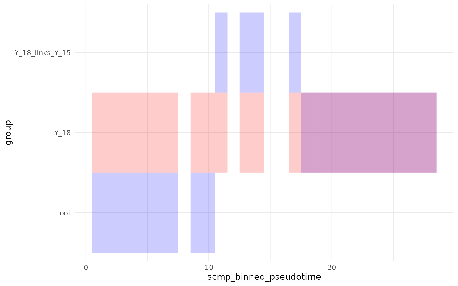
As we can see above, the tiles in red represent the original bins, while the blue represents the new bins “Y_18”. At the end, we also observe the overlap where the original bins of branch Y_18 are shifted to the end.
Pseudobulk
## Combine all metadata
new_binned_data <- rbind(Y_52_binned_data, Y_18_binned_data, Y_15_binned_data)

## Create a new object
multi_scmp_ob_A_manual <- multi_scmp_ob_A

## Update dense Metadata slot
cDense(multi_scmp_ob_A_manual) <- new_binned_data

## Set the group used for binning
multi_scmp_ob_A_manual@Parameters@path_col <- "group2"

## Perform Aggregation
multi_scmp_ob_A_manual <- pb_counts(
  scmpObj = multi_scmp_ob_A_manual,
  assay_name = "counts",
)

## Plot
plotBinTile(multi_scmp_ob_A_manual)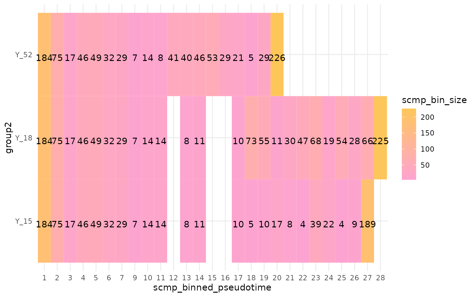
From scMaSigPro version 0.0.4 onwards, a
wrapper function was introduced to assist in ordering the bins. The
working of the wrapper function sc.restruct() is shown
below, and it works on fairly simplified datasets like the one
demonstrated in this vignette.
Reorder Bins with sc.restruct()
## Showcase sc.restruct wrapper
multi_scmp_ob_B <- sc.restruct(multi_scmp_ob_A,
  end_node_list = list("Y_15", "Y_18", "Y_52"),
  root_node = "root", link_node_list = list("Y_18_links_Y_15"),
  verbose = FALSE, link_sep = "_links_", assay_name = "counts", aggregate = "sum"
)
# Show the new path
plotBinTile(multi_scmp_ob_B)
As we see in the plot above, the sc.restruct() wrapper
function performs the exact transformations internally. For future
updates (CRAN version), we will offer a Shiny-based solution that can
effectively handle more complicated datasets. However, as of
scMaSigPro version 0.0.4, users are required
to either use sc.restruct() or manually order the
datasets.
Running Workflow
# Polynomial Degree 2
multi_scmp_ob_B <- sc.set.poly(multi_scmp_ob_B, poly_degree = 3)

# Detect non-flat profiles
multi_scmp_ob_B <- sc.p.vector(
  multi_scmp_ob_B,
  verbose = FALSE
)

# Model refinement
multi_scmp_ob_B <- sc.t.fit(
  multi_scmp_ob_B,
  verbose = FALSE
)

# Apply filter
multi_scmp_ob_B <- sc.filter(
  scmpObj = multi_scmp_ob_B,
  rsq = 0.5,
  vars = "groups",
  intercept = "dummy",
  includeInflu = TRUE
)

# Plot upset
plotIntersect(multi_scmp_ob_B)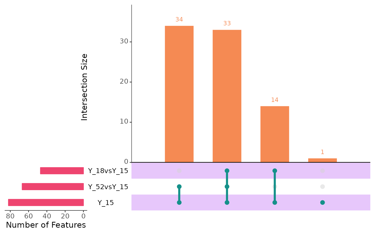
Now, in the above scenario, Y_15 is treated as the reference, and we will look at the genes that are expressed differently compared to this branch. This approach will help us understand how genes are changing across the branches while considering the root cells for each of the downstream branches.
Significant Genes
## Perform Clustering
multi_scmp_ob_B <- sc.cluster.trend(multi_scmp_ob_B,
  k = 4, cluster_method = "kmeans"
)

## Plot Clusters
plotTrendCluster(multi_scmp_ob_B, verbose = FALSE)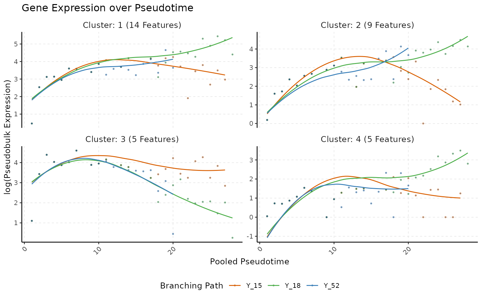
Session Info
sessionInfo(package = "scMaSigPro")## R version 4.3.0 (2023-04-21)
## Platform: x86_64-pc-linux-gnu (64-bit)
## Running under: Ubuntu 20.04.5 LTS
##
## Matrix products: default
## BLAS: /usr/lib/x86_64-linux-gnu/blas/libblas.so.3.9.0
## LAPACK: /usr/lib/x86_64-linux-gnu/lapack/liblapack.so.3.9.0
##
## locale:
## [1] LC_CTYPE=en_US.UTF-8 LC_NUMERIC=C
## [3] LC_TIME=es_ES.UTF-8 LC_COLLATE=en_US.UTF-8
## [5] LC_MONETARY=es_ES.UTF-8 LC_MESSAGES=en_US.UTF-8
## [7] LC_PAPER=es_ES.UTF-8 LC_NAME=C
## [9] LC_ADDRESS=C LC_TELEPHONE=C
## [11] LC_MEASUREMENT=es_ES.UTF-8 LC_IDENTIFICATION=C
##
## time zone: Europe/Madrid
## tzcode source: system (glibc)
##
## attached base packages:
## character(0)
##
## other attached packages:
## [1] scMaSigPro_0.0.4
##
## loaded via a namespace (and not attached):
## [1] bitops_1.0-7 gridExtra_2.3
## [3] rlang_1.1.3 magrittr_2.0.3
## [5] RcppAnnoy_0.0.22 matrixStats_1.2.0
## [7] e1071_1.7-14 compiler_4.3.0
## [9] mgcv_1.9-1 venn_1.11
## [11] systemfonts_1.0.5 vctrs_0.6.5
## [13] stringr_1.5.1 pkgconfig_2.0.3
## [15] crayon_1.5.2 fastmap_1.1.1
## [17] XVector_0.42.0 ellipsis_0.3.2
## [19] labeling_0.4.3 utf8_1.2.4
## [21] promises_1.2.1 rmarkdown_2.25
## [23] grDevices_4.3.0 UpSetR_1.4.0
## [25] ragg_1.2.7 purrr_1.0.2
## [27] xfun_0.42 zlibbioc_1.48.0
## [29] cachem_1.0.8 graphics_4.3.0
## [31] GenomeInfoDb_1.38.6 jsonlite_1.8.8
## [33] highr_0.10 later_1.3.2
## [35] DelayedArray_0.28.0 terra_1.7-71
## [37] parallel_4.3.0 R6_2.5.1
## [39] bslib_0.6.1 stringi_1.8.3
## [41] parallelly_1.37.0 GenomicRanges_1.54.1
## [43] jquerylib_0.1.4 assertthat_0.2.1
## [45] Rcpp_1.0.12 bookdown_0.37
## [47] SummarizedExperiment_1.32.0 knitr_1.45
## [49] IRanges_2.36.0 splines_4.3.0
## [51] httpuv_1.6.14 Matrix_1.6-5
## [53] igraph_1.6.0 tidyselect_1.2.0
## [55] rstudioapi_0.15.0 abind_1.4-5
## [57] yaml_2.3.8 codetools_0.2-19
## [59] admisc_0.34 plyr_1.8.9
## [61] lattice_0.22-5 tibble_3.2.1
## [63] Biobase_2.62.0 shiny_1.8.0
## [65] withr_3.0.0 evaluate_0.23
## [67] base_4.3.0 desc_1.4.3
## [69] proxy_0.4-27 mclust_6.0.1
## [71] pillar_1.9.0 BiocManager_1.30.22
## [73] MatrixGenerics_1.14.0 stats4_4.3.0
## [75] plotly_4.10.4 generics_0.1.3
## [77] RCurl_1.98-1.14 S4Vectors_0.40.2
## [79] ggplot2_3.5.1 munsell_0.5.0
## [81] scales_1.3.0 BiocStyle_2.30.0
## [83] stats_4.3.0 xtable_1.8-4
## [85] class_7.3-22 glue_1.7.0
## [87] lazyeval_0.2.2 tools_4.3.0
## [89] datasets_4.3.0 data.table_1.15.0
## [91] fs_1.6.3 grid_4.3.0
## [93] utils_4.3.0 tidyr_1.3.1
## [95] methods_4.3.0 colorspace_2.1-0
## [97] SingleCellExperiment_1.24.0 nlme_3.1-164
## [99] GenomeInfoDbData_1.2.11 cli_3.6.2
## [101] textshaping_0.3.7 fansi_1.0.6
## [103] S4Arrays_1.2.0 viridisLite_0.4.2
## [105] dplyr_1.1.4 gtable_0.3.4
## [107] sass_0.4.8 digest_0.6.34
## [109] BiocGenerics_0.48.1 SparseArray_1.2.4
## [111] farver_2.1.1 htmlwidgets_1.6.4
## [113] memoise_2.0.1 maSigPro_1.74.0
## [115] entropy_1.3.1 htmltools_0.5.7
## [117] pkgdown_2.0.7 lifecycle_1.0.4
## [119] httr_1.4.7 mime_0.12
## [121] MASS_7.3-60We extracted the vertex from UMAP and the trajectory was learned on tSNE. This is because our CDS object has the tSNE coordinates stored in the UMAP slot. This was done because
monocle3::learn_graph()does not work with tSNE coordinates. You can read more about this issue on monocle3-issues/242↩︎